
Views: 19 Author: Site Editor Publish Time: 2026-08-18 Origin: Site
Accurate cycle time calculation goes far beyond a basic math exercise. It forms the ultimate foundation for underground mine profitability and capital expenditure decisions. Planners rely on these numbers daily. Operations live or die by their accuracy.
Underground environments present unique operational constraints. You face steep declines, tight single-lane drifts, and frequent passing bay delays. Ventilation stops and rough terrain make standard surface-mining calculations completely inadequate. You simply cannot divide distance by average speed here. Localized traffic congestion constantly disrupts theoretical travel times.
This guide shows how operational leaders can transition from estimated baselines to empirical data models. You will learn to optimize your haulage fleet planning and manage material handling contracts effectively. We explore fundamental formulas, hidden bottlenecks, and the modern technologies necessary to capture operational reality.
Formula Breakdown: Total cycle time equals fixed times (loading, dumping, maneuvering) plus variable times (loaded haul, empty return, conditional delays).
Underground Constraints: Accurate models must account for passing bay wait times, gradient shifts in declines, and localized traffic congestion.
Equipment Matching: Optimizing loader-to-truck ratios is critical; an unbalanced fleet guarantees either loader idle time or truck queuing.
Technology Shift: Transitioning from manual time-studies to Fleet Management Systems (FMS) or telematics is necessary for scalable, real-time mine truck productivity calculation.
A minor miscalculation in your assumptions creates massive downstream consequences. Consider a margin of error as small as 5% in your baseline cycle time. Over a long shift, this discrepancy compounds rapidly. If you overestimate efficiency, you under-fleet your operation. This leads directly to missed production targets. Conversely, underestimating efficiency causes over-fleeting. You waste critical capital expenditure on unnecessary machinery.
Precise baseline data heavily influences contracting and commercial value. Many operations rely on third-party haulage contractors. Ambiguous cycle times complicate these agreements. Accurate mine truck productivity calculation allows you to establish fair cost-per-tonne estimates. You gain immense leverage during contract negotiations. Both parties benefit from transparent, data-backed operational expectations.
Granular time tracking also isolates hidden operational bottlenecks. Fleet managers often blame trucks for low production. However, detailed cycle data tells a different story. You might discover severe crusher queues rather than slow driving speeds. You may find inefficient loading setups causing extreme spotting delays. Identifying the exact failure point lets you apply targeted solutions. You stop guessing and start optimizing.
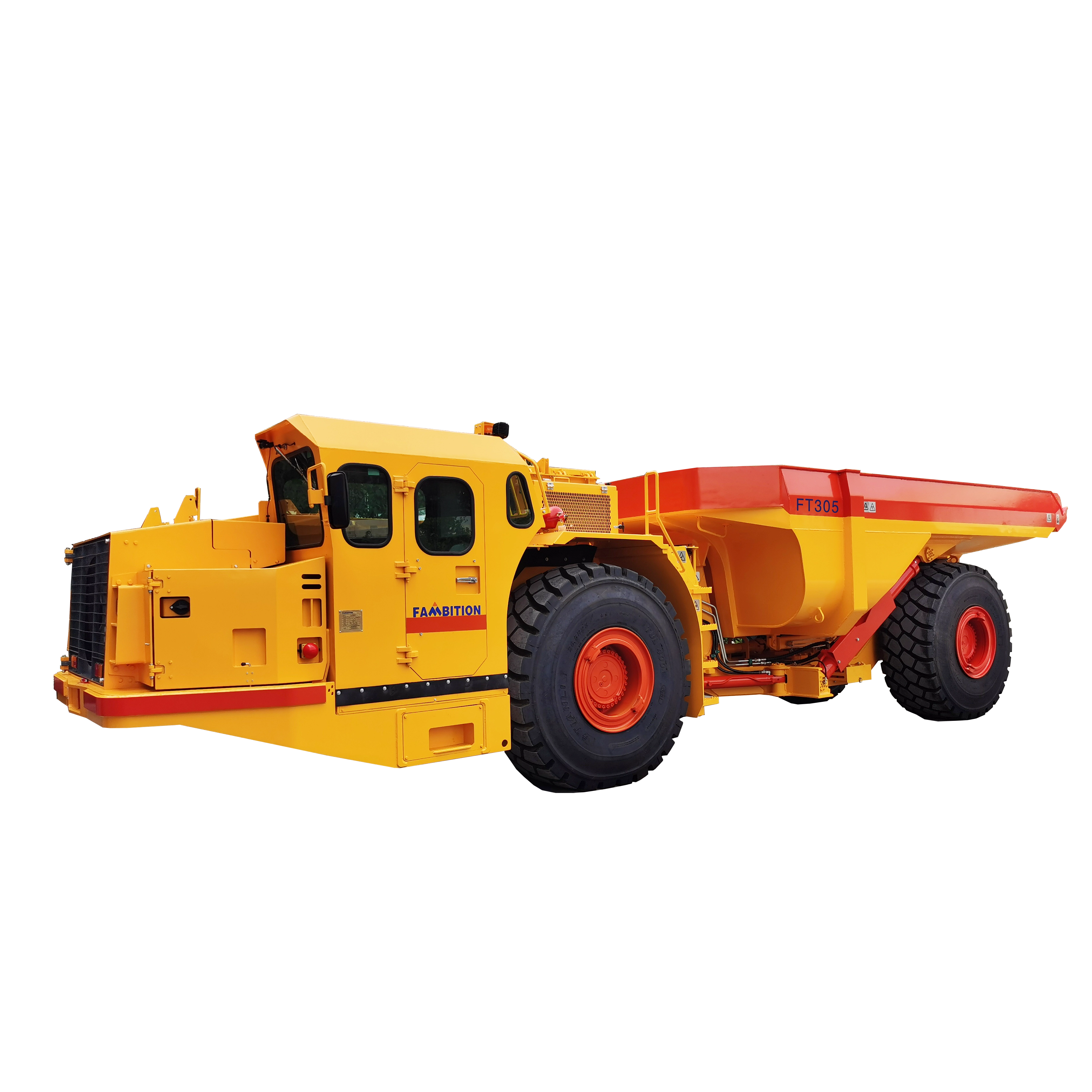
You must break down the haul cycle into measurable components. We divide these into fixed times, variable times, and underground-specific modifiers.
Fixed times occur regardless of haul distance. They involve distinct stationary activities.
Spotting and loading represent the first fixed phase. Operators take time to position vehicles safely under the loader or ore chute. Once in place, the machine receives its payload. Dumping and maneuvering form the second fixed phase. Drivers must reverse into position at the ore pass, crusher, or stockpile. They dump the load, lower the tray, and clear the immediate area.
Variable times depend strictly on distance, speed, and terrain.
Loaded travel time requires complex analysis. You must factor in high rolling resistance and steep gradients. Most decline ramps run at 1:7 or 1:8 slopes. Gravity heavily limits loaded vehicle speeds. Empty travel time calculates the return trip. The machine moves faster, but you must strictly note site speed limits and equipment braking constraints.
Surface mining ignores localized delays. Underground mining must embrace them.
Unavoidable modifiers ruin perfect mathematical models. Drivers wait at passing bays for oncoming traffic. They stop to clear mandatory ventilation doors. They often face interference from remote-bogging operations. You must build these conditional delays into your core formula.
| Cycle Phase | Component Type | Key Influencing Factors |
|---|---|---|
| Spotting & Loading | Fixed Time | LHD bucket size, operator skill, loading area width |
| Dumping & Clearing | Fixed Time | Crusher availability, stockpile space, tray lift speed |
| Loaded Travel | Variable Time | Ramp gradient, rolling resistance, engine power |
| Empty Return | Variable Time | Braking capacity, speed limits, ramp conditions |
| Conditional Delays | Modifier | Passing bays, vent doors, shift changes |
An unbalanced fleet destroys operational efficiency. You must perfectly match your loaders with your hauling equipment.
You need the optimal number of loader passes to fill the underground truck. Too many passes waste time. Too few passes cause under-loading. Spillage occurs if the match is mathematically incorrect. Follow these precise steps for pass-matching:
Determine the exact target payload of the hauling unit.
Calculate the actual loose material payload of the LHD bucket.
Divide the truck payload by the LHD payload.
Analyze the result to ensure it lands near a whole number (typically 3 to 5 passes).
Adjust bucket sizes or vehicle capacities if the ratio falls outside optimal ranges.
You constantly face a trade-off between loader wait time and queue time. Queueing theory helps you balance this equation. If you deploy too many hauling units, they queue at the loader. Capital sits idle. If you deploy too few, the loader waits. Production drops. You must calculate the exact intersection where both machines maintain high utilization rates.
Success criteria depend on matching bucket capacities with cycle times. You look at Load-Haul-Dump (LHD) units alongside articulated or rigid vehicles. The math must align. A massive LHD paired with a small hauling unit causes immediate bottlenecking. Fleet managers evaluate these ratios continuously to guarantee smooth material flow.
How you measure data dictates the quality of your planning. The industry currently straddles two vastly different measurement methodologies.
Traditional manual time-and-motion studies rely on stopwatches and clipboards. Planners stand in the dirt, logging times manually. Modern approaches utilize Fleet Management Systems (FMS) and IoT telematics. These systems pull live data directly from the machine's onboard computers.
Static spreadsheet calculators fail as mine topographies change. A spreadsheet assumes road conditions remain perfect. It assumes traffic flows freely. This is dangerous. Dynamic software tools, such as Alastri or Micromine, adjust to real-time variables. They scale effortlessly across multiple levels and expanding decline networks.
Fleet managers must shortlist FMS solutions carefully. Look for these crucial dimensions:
Integration Capability: The system must connect seamlessly with your existing dispatch and planning platforms.
Offline Data Buffering: Underground environments contain extensive dead-zones. The software must buffer data offline and sync upon returning to network coverage.
Reporting Clarity: Dashboards should highlight actionable bottlenecks immediately, rather than just dumping raw data.
Hardware Durability: Sensors must withstand extreme heat, moisture, and vibration.
Theoretical calculations often fail upon execution. You must anticipate the gap between mathematical models and operational reality.
You plan for optimal conditions, but reality delivers chaos. Deteriorating road conditions drastically reduce travel speeds. Deep ruts and standing water ruin rolling resistance. Operator skill variance also skews your data. A highly skilled driver completes a cycle much faster than a novice. Furthermore, poor fragmentation creates awful bucket fill factors. If the blast yields oversized rocks, loading takes twice as long.
Never assume 100% nominal payload. This represents a massive implementation risk. You must calculate the actual loose density of the ore. You must apply accurate swell factors. Solid rock expands when blasted. A 40-tonne capacity vehicle rarely carries exactly 40 tonnes of blasted material. Relying on manufacturer brochures instead of actual material density ruins your cycle time math.
You need a continuous feedback loop. Audit your software outputs against physical shift reports weekly. If the software predicts 25 loads but the shift delivers 18, investigate the variance immediately. Refine your planning assumptions based on this ongoing audit process. Treat cycle time as a living metric.
| Risk Factor | Impact on Cycle Time | Recommended Mitigation |
|---|---|---|
| Poor Road Maintenance | Increases variable travel time by 10-20% | Schedule routine grader passes on main declines |
| Oversized Fragmentation | Prolongs spotting and loading fixed times | Optimize drill and blast parameters |
| Payload Overestimation | Reduces actual tonnes moved per hour | Conduct regular material swell and density tests |
| Operator Inexperience | Creates inconsistent cycle durations | Implement targeted simulator training programs |
Accurate cycle time calculation represents a continuous process, not a one-off math problem. You must constantly adapt your formulas to match changing mine conditions. Relying on static spreadsheets will eventually cost your operation money.
To improve your efficiency, audit your current baseline data immediately. Take a hard look at your existing loader-truck pairings to ensure pass-matching remains optimal. Finally, request proofs-of-concept from FMS vendors. Bridging the gap between theoretical calculations and operational reality requires modern telematics. Act on your data, refine your assumptions, and watch your cost-per-tonne drop.
A: Acceptable queue time generally falls between 10% and 15% of the total cycle time. However, this heavily depends on fleet size. Smaller fleets aim for near-zero queue times to maximize machine utilization. Larger fleets tolerate slightly higher queue times to ensure the loader never sits idle.
A: Gradient changes severely impact speed due to gravity and gear-limiting. When navigating a steep 1:7 decline, the transmission automatically locks into a lower gear. This prevents engine overspeed but drastically reduces uphill travel velocity. Even a 2% gradient increase can double the required rimpull.
A: No. Surface calculators fail in underground environments. They ignore critical underground-specific constraints. Surface formulas do not account for single-lane drift traffic, mandatory passing bay waits, or ventilation door delays. Using them guarantees inaccurate baselines and flawed capital expenditure models.
A: You should recalculate baselines dynamically, but formal reviews must occur during major operational triggers. Recalculate whenever you advance to a new level, change fleet composition, or alter the fundamental mine plan. Quarterly audits provide a strong safeguard against unnoticed efficiency drops.
 English


